The topic TurboQuant tackles the hidden memory problem that’s been limiting your local… is currently the subject of lively discussion — readers and analysts are keeping a close eye on developments.
This is taking place in a dynamic environment: companies’ decisions and competitors’ reactions can quickly change the picture.
If you’ve spent any time running local LLMs, you’ve probably hit the same wall I have. You find the perfect model quantized to 4-bits, just small enough to fit in your GPU’s context window. You then load it up, only to watch as you run out of available memory the moment you try to do anything with a context window longer than 10 tokens. The model fits, but the part that allows you to actually have a conversation doesn’t.
Weight quantization has gotten most of the mainstream attention, and for good reason. Tools like GPTQ, AWQ, and the GGUF format in llama.cpp have come a long way to enable people to run even a 70B parameter model on a single GPU now if you’re willing to go low enough on precision. But here’s the thing: weight quantization only solves half the problem. The other half, the part that sometimes requires more memory than the model itself, is the KV cache. KV cache compression has been an active research area for a while, with methods like KIVI and others chipping away at the problem, but it’s been comparatively less mature and less standardized in local inference tooling.
Google’s TurboQuant algorithm looks to change that, and when you pair it with architectural changes like Gated DeltaNet, the picture for running large models locally starts to look very different.
When you quantize a model’s weights from FP16 down to 4-bit, you’re compressing the static part of the model; that is, the parameters that don’t change during inference. A 70B model goes from roughly 140GB down to about 35GB. That alone is what makes local LLMs practical on consumer hardware in the first place.
The KV cache is a different problem entirely. During inference, every attention layer stores a key and value vector for each token it processes so it doesn’t have to recompute them on future tokens. The memory required follows a straightforward formula:
2 * layers * KV_heads * head_dim * sequence_length * bytes_per_element
The factor of 2 accounts for both the key and value tensors. This grows linearly with context length, and depending on the model’s architecture, it can get really large, really fast.
How large exactly, though, typically depends on whether the model uses Multi-Head Attention (MHA) or Grouped Query Attention (GQA). With MHA, every attention head has its own set of keys and values. Take Llama 2 7B as an example: it has 32 layers, 32 KV heads, and a head dimension of 128. Its native context window is only 4K tokens, but if you were to extend it to 128K (as community projects with YaRN have done), the KV cache alone would consume about 64GB in FP16. That’s more than many GPUs can hold, and that’s before you account for the model weights.
Modern models have largely moved to GQA, which shares KV heads across multiple query heads. Llama 3.1 8B, for example, uses only 8 KV heads instead of 32, which cuts the KV cache to roughly 16GB at the same 128K context. That’s a big improvement, but it’s still a lot of memory that weight quantization doesn’t touch. At shorter context lengths, you’re looking at about 1GB per 8K tokens for a GQA model like Llama 3.1 8B, and that adds up quickly once you start doing anything meaningful with longer conversations or large codebases.
This is why so many local LLM users find themselves capping their context window at 32K or 64K tokens, even when the model technically supports 128K or more. The model fits, but the conversation memory doesn’t.
TurboQuant, which Google will present at the International Conference on Learning Representations 2026 (ICLR 2026), is a two-stage compression algorithm for quantizing the KV cache. Before getting into how it works, here’s what it achieves: the paper reports KV cache compression exceeding five-times at its most aggressive 2.5-bit setting, with what the Google blog describes as “perfect downstream results across all benchmarks” in needle-in-haystack tests. The blog also claims up to eight-times speedup in attention computation on H100 GPUs. At the lossless 3.5-bit setting, compression is closer to 4.6x versus FP16, which is still a lot of reclaimed memory. And it requires zero calibration, meaning it works on any model instantly with no offline preparation. according to the data the paper, it achieves “absolute quality neutrality” at 3.5 bits per channel and “marginal quality degradation” at 2.5 bits per channel. The Google Research blog rounds this to “3 bits” in its headline, but the paper’s own numbers are more precise, and the difference does actually matter.
So how does it pull this off? The first stage is called PolarQuant, and the idea behind it builds on a technique that has already conceptually proven itself in weight quantization. Methods like QuiP# showed that multiplying weight matrices by random orthogonal transforms before quantizing them “spreads out” the values, removing the outlier-heavy structure that makes low-bit quantization difficult. PolarQuant applies a related random-rotation idea to the KV cache. It’s a hard concept to get your head around, but it’s quite simple once you understand it.
Normally, when you compress a block of numbers, you need to store extra metadata for each block: a scale factor and a zero-point that tell the decoder how to interpret the compressed values. These constants typically use up one or two extra bits per value, which partially defeats the purpose of compressing in the first place. PolarQuant gets around this by first multiplying the input vectors by a random rotation matrix. This doesn’t destroy any of the relationships in the data, but it exploits a property of high-dimensional geometry: after rotation, the coordinates become well-behaved enough that simple scalar quantization works near-optimally.
Think of it like stirring a pot until the ingredients are evenly distributed. You haven’t changed how much of each ingredient is there, but you’ve mixed them into a regular enough form that the same measuring cup works for every batch. The rotation makes the data statistically uniform based on the vector’s dimension alone, not the actual data. Because the distribution is known in advance, optimal compression codebooks can be precomputed and reused everywhere, without the need for per-block metadata. In other words, you can eliminate the one or two bits of extra overhead entirely.
The second stage cleans up the small errors left by PolarQuant. It’s called QJL (Quantized Johnson-Lindenstrauss), and it applies a random projection to the residual and then crushes each coordinate down to a single sign bit: a positive or negative value of one, and this costs one additional bit per channel. The reason this matters for attention specifically is that accuracy depends on the relationship between the cached key and the incoming query. QJL only quantizes the cached key to a sign bit, while the query vector stays at high precision when computing attention scores. As the Google blog puts it, QJL “balances a high-precision query with the low-precision, simplified data.” Quantizing both sides would introduce systematic bias in the attention scores. Keeping one side precise is what avoids that.
What makes this different from existing weight quantization methods is that no preparation is needed. GPTQ analyzes how sensitive each weight is to rounding errors; AWQ observes activation patterns to identify important weights. Both need offline calibration passes with sample data. TurboQuant needs none of that. It’s data-oblivious, meaning the codebooks and random projections work on any vector from any model instantly. The paper tested on Llama 3.1 8B Instruct and Ministral 7B Instruct (the Google blog also cites Gemma results).
The paper also proves that TurboQuant operates within a factor of approximately 2.7x of the information-theoretic lower bound on quantization distortion, the absolute minimum from Shannon’s rate-distortion theory. No quantizer can beat that bound under the paper’s distortion framework, and getting within 2.7x of it while being fully data-oblivious and processing vectors one at a time is genuinely impressive.
Put simply: a GQA model like Llama 3.1 8B generating 16GB of KV cache at 128K context in FP16 would drop to roughly 3GB at 2.5 bits with TurboQuant (over five-times compression), or about 3.5GB at 3.5 bits (just over four-and-a-half times). For a full-MHA model like Llama 2 7B, the 64GB baseline would compress to somewhere in the range of 12-14GB. That’s a pretty big difference.
TurboQuant compresses the KV cache, but there’s another approach that eliminates the need for much of it in the first place. Gated DeltaNet is a linear attention mechanism that replaces standard self-attention with a fixed-size recurrent state. It doesn’t grow with context length at all.
Think of standard attention as a filing cabinet where you keep a separate folder for every token you’ve ever seen. That’s the KV cache, and it grows with every new token. Standard linear attention tries to compress this into a single summary matrix, but it does so by blindly piling new information on top of old information with no way to correct mistakes or forget irrelevant details.
DeltaNet takes a smarter approach. Instead of just stacking new associations onto the state, it checks what the state currently “remembers” about a given key and only corrects the difference between that and the new value. This is called the delta rule, borrowed from classical neural network learning theory. It means the state is constantly self-correcting rather than blindly accumulating.
Gated DeltaNet (the variant used in production models) adds a forgetting mechanism on top of this. A learned decay gate controls how quickly old information fades from the state. When the gate is close to 0, the state rapidly forgets. When it’s close to 1, the state holds onto everything. There’s also an output gate for controlling what information actually gets passed forward. The result is a fixed-size state matrix per layer, with dimensions n_heads * d_head * d_head, and this size never changes no matter how many tokens you’ve processed. That’s the key part: it has constant memory, regardless of context length.
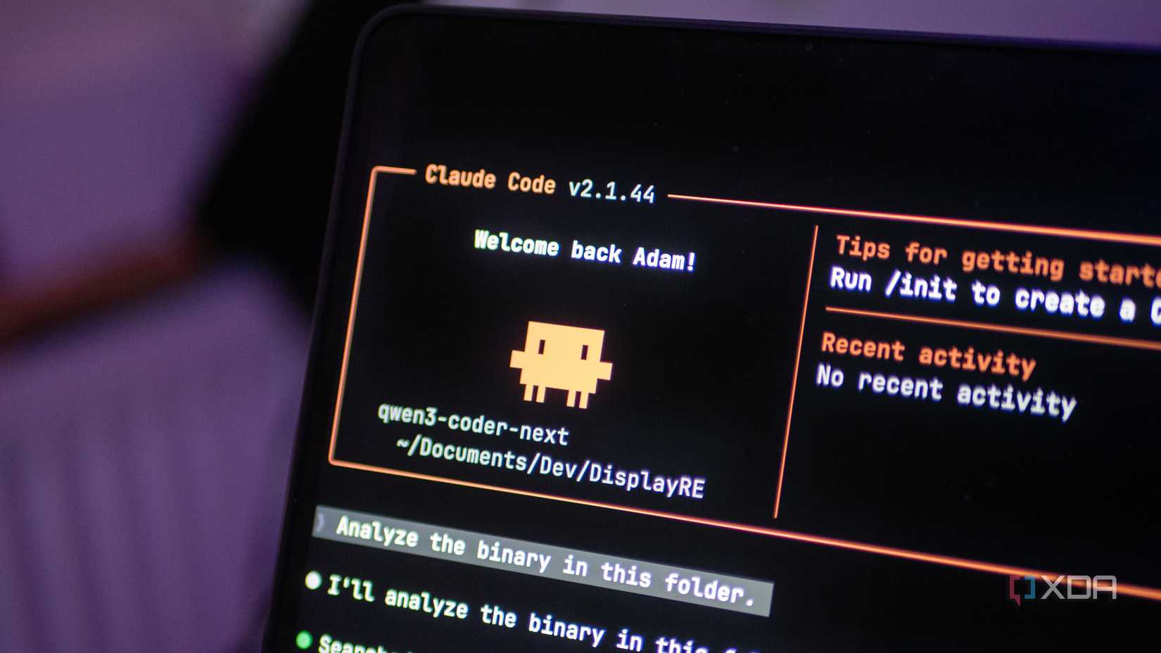
I’ve seen what this makes possible thanks to Qwen3-Coder-Next, which I’ve run on the Lenovo ThinkStation PGX. It has 128GB of unified memory shared between its Arm CPU and Blackwell GPU, and I’ve been able to maintain a 170,000-token context window with the model running at FP8. That’s an 80B parameter model (with only 3B active per token across its 512 experts in a Mixture-of-Experts architecture) holding 170K tokens of context. So, we’ve gone from a theoretical 64GB FP16 context-length using Llama 2 with YaRN scaling, to just a few gigabytes at a much larger context length. And DeltaNet is a big part of why that’s possible.
Qwen3-Coder-Next uses a three-to-one hybrid architecture across its 48 layers, with 12 repeating cycles of three Gated DeltaNet blocks followed by one full-attention block. That means 36 of 48 layers use DeltaNet’s fixed-size state instead of a growing KV cache. Only the 12 full-attention layers generate KV cache entries, and those use aggressive GQA with just 2 KV heads and a head dimension of 256, keeping each layer’s cache compact.
The DeltaNet layers have a completely different head configuration: 16 QK heads and 32 value heads, both with a smaller head dimension of 128. The 16 key heads are expanded to match the 32 value heads before the delta rule computation, and going back to our earlier formula, this gives us:
This means that all 36 DeltaNet layers combined come in at about 18MB of fixed state. If those 36 layers used full attention instead, each one would need its own growing KV cache. Instead, they use 18MB total, and that number stays the same whether you’re at 1K tokens or 170K.
The 12 full-attention layers still generate a KV cache that grows with context, and the exact cost in practice depends on your precision and how your inference engine manages the hybrid architecture. vLLM, for example, uses a paged memory system with a hybrid KV/state manager that tunes logical block sizes so full-attention and linear-attention states align in physical memory. Managing two fundamentally different layer types isn’t trivial, but the principle is what matters: 75% of the model’s layers contribute effectively nothing to the memory footprint as context grows, while the remaining 25% benefit from aggressive GQA with just 2 KV heads (compared to 8 in Llama 3.1 70B). The developers could afford that aggressive GQA precisely because most layers don’t need a KV cache at all.
Applying our earlier formula, 2 * layers * KV_heads * head_dim * sequence_length * bytes_per_element, we get the following values for just the full-attention layers:
If we want to calculate for FP16, we increase bytes-per-element to two. This doubles both values, but still uses very little memory overall.
The catch is that those 36 DeltaNet layers are working from a compressed summary of the conversation rather than a complete record. Each head’s 128*128 matrix is trying to represent 170,000 individual key-value pairs’ worth of context. It’s lossy by nature, which is why the model still needs those 12 full-attention layers. Those layers can handle precise retrieval.
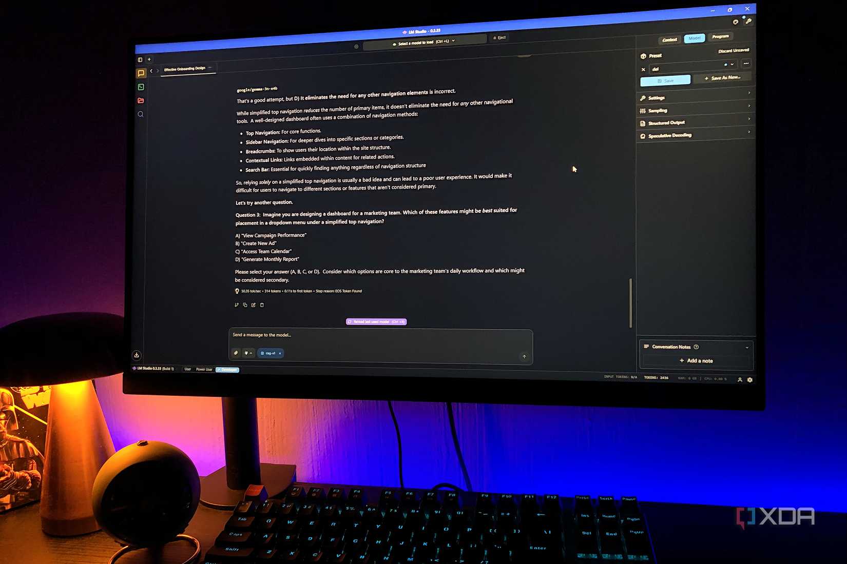
Kimi Linear from Moonshot AI takes a similar hybrid approach but refines DeltaNet with what it calls KDA (Kimi Delta Attention). The key difference is in the decay gate: where Qwen3-Coder-Next uses a scalar decay per attention head (one forgetting rate shared across all dimensions), KDA uses channel-wise gating, a separate decay rate for each feature dimension within a head. This means the model can retain long-range information in some dimensions while rapidly cycling short-term information in others within the same head. It’s a more expressive memory mechanism, and benchmarks show it converges faster on sequence reasoning tasks.
The tradeoff you’re making with any of these approaches is that DeltaNet compresses past context into a fixed-size hidden state. Unlike full attention, which can look back at any previous token directly, the DeltaNet layers can only access what their compressed state has retained. That’s why the hybrid ratio exists. You still need those full-attention layers to maintain the model’s ability to reason over specific details from earlier in the context. It’s not exactly free, but for long-context workloads, the memory savings are hard to ignore.
Here’s what excites me most about TurboQuant: it’s not an either-or proposition with approaches like DeltaNet. They operate on completely different parts of the inference pipeline. DeltaNet reduces how many layers need a KV cache. TurboQuant reduces how much memory the remaining KV cache layers consume. Stack them together, and the savings build on top of each other.
Take Qwen3-Coder-Next as an example. With its three-to-one hybrid architecture, only 12 of 48 layers generate KV cache. The raw KV cache for those layers is relatively small thanks to aggressive GQA, but in practice, inference engines like vLLM add overhead when managing hybrid architectures. TurboQuant could compress whatever KV cache remains: its ratios are measured against FP16 baselines, so the exact savings depend on what precision you’re starting from, but the approach is the same. Combined with just 18MB of fixed DeltaNet state across 36 layers, the total memory for runtime context would be a fraction of what a traditional architecture demands.
Compare that to what a traditional full-attention 80B model with full MHA heads would require at the same context length. Without GQA, without DeltaNet, without KV cache quantization, you’d be looking at tens of gigabytes of KV cache alone. Between architectural sparsity (MoE), linear attention (DeltaNet), aggressive GQA, and now effective KV cache quantization (TurboQuant), each of these chips away at a different part of the memory budget, and they all do some pretty heavy lifting.
For consumer hardware, this matters even more. A desktop with 24GB of VRAM running a 4-bit quantized model currently has to choose between model size and context length. With TurboQuant handling the KV cache and future models adopting DeltaNet-style hybrid architectures, that tradeoff becomes far less painful. You could run larger models and maintain longer contexts on the same hardware, because the memory that used to be consumed by the KV cache is now available for model weights or additional context.
Weight quantization made local LLMs possible to run on a standard consumer PC. GQA reduced the KV cache overhead. DeltaNet-style hybrid architectures cut it further by eliminating the cache from most layers entirely. And now TurboQuant compresses what remains to a mere 2.5 or 3.5 bits per channel with no calibration required. Each of these works on a different part of the memory budget, and none of them conflict with each other. The memory wall that’s kept local inference constrained is eroding from every angle, and if the trend holds, I think some larger models that currently need data center hardware will be running on desktop machines sooner than most people expect. That’s why i love TurboQuant and what it represents: it’s not what it does today, but what it could open up tomorrow.